The sound Doppler effect visualized in Mathematica and a measurement of g

This is an advanced demonstration that illustrates the following: Fourier transforming data, audio analysis and, more importantly, the Doppler effect. As a by-product of the method, a measurement of the acceleration of gravity g is made. The code can be found here.

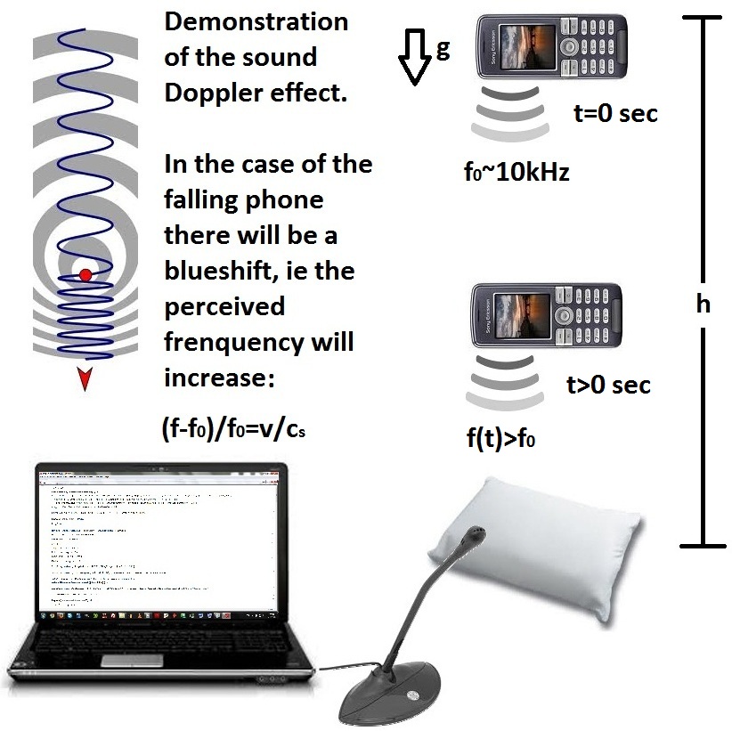
The whole idea is very simple and is illustrated in the Figure below. First make a sound file that contains a handful of known frequencies around 10kHz. Then, pass this file to your cellphone, play the sound and drop the phone from a small height (around 1m should do) on to a pillow or something soft. While the phone is falling record the sound with a mic on your laptop. If you then analyze the frequencies of the new file you should notice that they are shifted due to the Doppler effect! The relative shift of the frequencies is proportional to the velocity of the falling phone over the speed of sound.

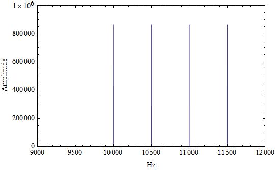
The power spectrum of the original sound file can be seen in the Figure below. The frequency spikes are sharply centered at 10, 10.5, 11 and 11.5 kHz.

The power spectrum of the recorded sound file can be seen in the Figure below. Only the two frequencies at 10 and 11 kHz are now visible, even though the recording was conducted in complete silence. The fact that it was a 5$ dirty cheap mic might have been a factor...

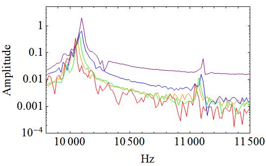
In order to simplify the analysis we split the recorded data into five bins of equal width and Fourier transform each bin seperately. The power spectrum in each case is shown below.

The measurements of the peak frequencies in each of the five bins are as follows:

$\begin{array}{cc}\mathrm{Channel\; 1}& \mathrm{Channel\; 2}\\ \mathrm{10044.715\; Hz}& \mathrm{11040.601\; Hz}\\ \mathrm{10061.885\; Hz}& \mathrm{11057.771\; Hz}\\ \mathrm{10079.056\; Hz}& \mathrm{11074.942\; Hz}\\ \mathrm{10096.226\; Hz}& \mathrm{11092.112\; Hz}\\ \mathrm{10096.226\; Hz}& \mathrm{11109.283\; Hz}\end{array}$

The measurements of the relative shifts $\mathrm{\delta f}/f_0$ in the frequencies in each of the five bins:

$\begin{array}{cc}\mathrm{Channel\; 1}& \mathrm{Channel\; 2}\\ 0.00447& 0.00369\\ 0.00619& 0.00525\\ 0.00791& 0.00681\\ 0.00962& 0.00837\\ 0.00962& 0.00993\end{array}$

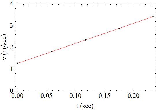
Unfortunately, in Channel 1, the last two measurements are duplicated, ie there was no shift in the frequencies, so we are left with only channel 2. Luckily, this turns out to work great. Next, since the phone is free-falling (lets ignore air resistance) we can fit the data to the following model $\mathrm{\delta f}/f_0=v\left(t\right)/c_s=\frac{v_0+gt}{c_s}$, where $v_0$ is the initial velocity, g is the acceleration of gravity and $c_s$ the speed of sound.

According to Wolfram Alpha, the speed of sound at an altitude of 667m, at which Madrid is approximately located, at a temperature of 22 C is 344.23m/s. With this we can fit the data, and the best-fit values are $v_0$=1.27 m/s and g=9.23 m/s^2. The latter is in especially good agreement with the theoretical value for g=9.80 m/s^2 considering:
a) the simplicity of the method,
b) that this is not supposed to be a real experiment (!) and
c) it was done in less than 5 minutes during a lazy afternoon...

A plot of the best-fit line along with the data is shown below. The initial non-zero velocity is due to the fact that the phone had already started falling before the sound file started playing. In any case, it doesn't affect the measurement of g which is the slope of the equation mentioned above.

Legal: The codes found in this page are provided with no warranty whatsoever and I'm in no way responsible for any loss of data, injury, harm to you or your equipment. Finally, everything is published under the GNU General Public License (GPLv3), found here.

Science warning: This is not supposed to be a real experiment, so please consider that before sending me angry emails asking why I didn't consider this or that effect, why there are no error bars in the best-fit parameters or that I should use some weird method to minimize the systematic errors...